Chapter 2 Environmental Valuation
Kolstad (2010, Chapters 7 & 10); Adamowicz et al. (1998)
Actions of firms—which are directed to maximize their profits, and often result in environmental pollution of some sort—are primarily motivated by consumer demand for goods offered by these firms. The demand functions tells us:
- how much a person will spend on a given good out of an array of options;
- the marginal valuation a consumer places on a good at different consumption levels; and
- how much of the good an individual is willing to forgo if the price increases.
Things are different with environmental goods, because there are no markets for those. For example, for an environmental good such as ‘clean air,’ we do not have information on different consumption levels at different prices, even though people who value clean air more would be willing to pay a higher price for an ‘additional unit’ of the air quality.
2.1 Willingness to Pay
Valuation (of a good) is an individual–specific measure that depicts the maximum amount of money a person would be willing to give up to obtain a unit amount of the good. For example, willingness to pay (WTP) for the environmental good (e.g., certain degree of air quality) is the dollar amount an individual is willing to give up, to obtain such air quality. WTP is the amount which, if paid in exchange for a good or service, leaves a person just as well off as without paying and without receiving the good or service. The concept of the WTP for environmental quality is closely linked with the concept of damages due to the reduction of environmental quality.
2.2 Measuring Demand for Environmental Goods
Two basic approaches to measuring demand rely on revealed preferences and stated preferences. In revealed preference, the actual choices are observed, which allows us to infer the values of environmental goods. The usual ‘problem’ with this approach is that, it is not directly applicable to goods for which markets do not exist (e.g., most environmental goods).
In stated preference, the actual choice is not observed, rather people are asked to report (state) how they would trade-off money for the good if they were to face such a choice. Thus, the stated preference method allows us to directly examine individuals’ valuation for goods and services for which markets do not exit. The issue with this approach is with the hypothetical nature of information—when asked, people may understate or overstate their valuation for some strategic reasons or simply due to the carelessness.
2.3 Revealed Preferences
Even though markets rarely exist for environmental goods, the observed demand for market goods in different ‘environmental scenarios’ may help us with the valuation of environmental goods.
2.3.1 Hedonic Method
Consider housing as an example of a market good, \(x\), and air quality as an environmental good, \(e\). Let \(p_x\) denote the housing price. The goal is to infer the value of the environmental good. The relationship between the housing prices, air quality and quantity of housing demanded can be given by: \(x=h(p_x,e)\); that is, the demand for housing is a function of its price, as well as the air quality in the neighborhood. Turns out, such demand function can help us understand the demand for the environmental good, which is equivalent to marginal WTP of \(e\).
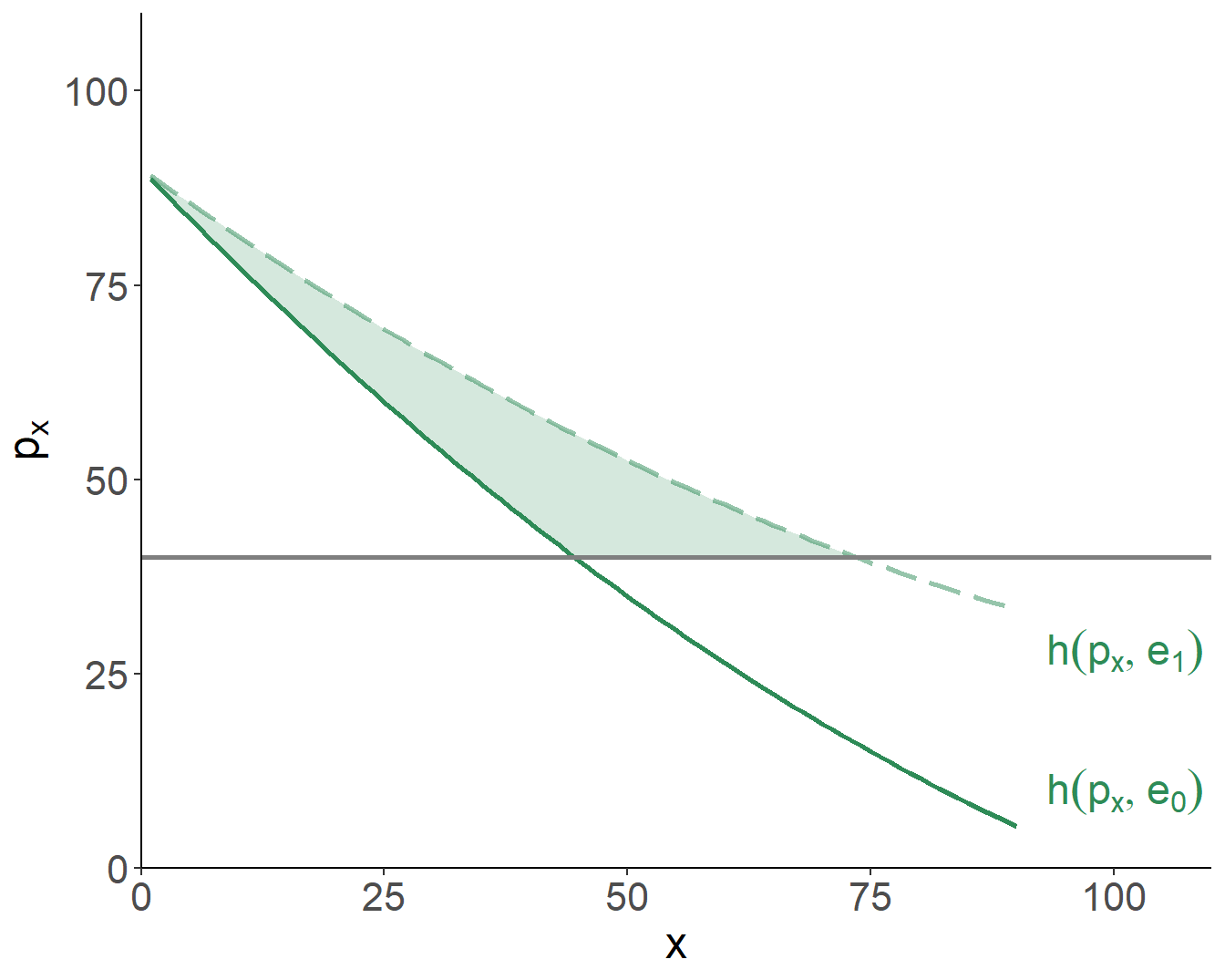
Figure 2.1: WTP for Clean Air
If the only purpose of the air quality were to enhance the experience of consuming the market good in consideration, the foregoing analysis addresses the question of obtaining demand for an environmental good. But air quality surely affects individuals’ well-being in ways unrelated to housing. So, the ‘estimated’ value of the environmental good is, really, a lower bound—only a portion of total value attached to the air quality is captured. An additional challenge, in such analysis, is accounting for all other factors that affect housing demand.
2.3.2 Travel Cost Method
Travel cost method infers values of environmental goods by examining costs that visitors incur getting to a recreational site and then using this information to estimate willingness to pay that site.
As another example, consider a range of recreational sites located at some distance from a city. People travel to these sites with different levels of environmental amenities. When they do so, they incur different costs (costs of transportation; membership/entrance fees; opportunity costs of time). Thus, people’s demand for environmental good (available at these recreational sites) can be inferred from costs they incur in the process.
2.4 Stated Preferences
Demand for a range of environmental goods may not be examined using (previously discussed) revealed preference methods. Existence value, for example, is very difficult (if not impossible) to estimate based on actual behavior of individuals, because their choices with regard to market goods are unaffected by whether or not ‘that something’ is available. Moreover, for many environmental goods, there is no market for ordinary goods, through which their value can be reflected. This has motivated researchers to develop valuation techniques that involve the construction of a market, when such market is absent.
Two broad categories of constructed markets exist: hypothetical and experimental. Valuation though hypothetical constructed markets is referred to as stated preference, or contingent valuation. In such hypothetical scenarios, potential consumers are asked to state their valuation of a good, if there were a market for such good (hence the term ‘contingent’).
In the case of the experimental constructed markets, a researcher constructs all the (desired) characteristics of a market, and then observes participant’s behavior within this market. In the case of choice experiment, for example, a researcher presents a respondent with a choice of scenarios, with a price tag attached to each scenario, and a respondent chooses the preferred option; the choice set typically includes the the status quo (i.e., the ‘no change’) option as well.
2.5 WTP vs WTA
Thus far we have focused on WTP—the dollar amount someone would be willing to give up to obtain something. Another related and relevant measure is willingness to accept (WTA)—the dollar amount someone would be willing to accept in compensation for giving up something. Conceptually, WTP and WTA seem to be ‘mirror images’ of some sort: how much will an individual pay to live in a neighborhood with less air pollution vs. how much of a compensation will an individual accept to live in a neighborhood with more air pollution. Theoretically (as well as in practice), these two measures are not necessarily identical, however.
Consider an environmental good, \(e\), and a market good, \(x\). Let a starting bundle be \(\{x_0,e_0\}\), yielding utility: \(U_0 = U(x_0,e_0)\). Consider also an alternative bundle, \(\{x_0,e_1\}\), yielding utility: \(U_1 = U(x_0,e_1)\). We are interested in two measures:
- starting at \(e_0\), the WTP to move to \(e_1\); and
- starting at \(e_1\), the WTA to move to \(e_0\).
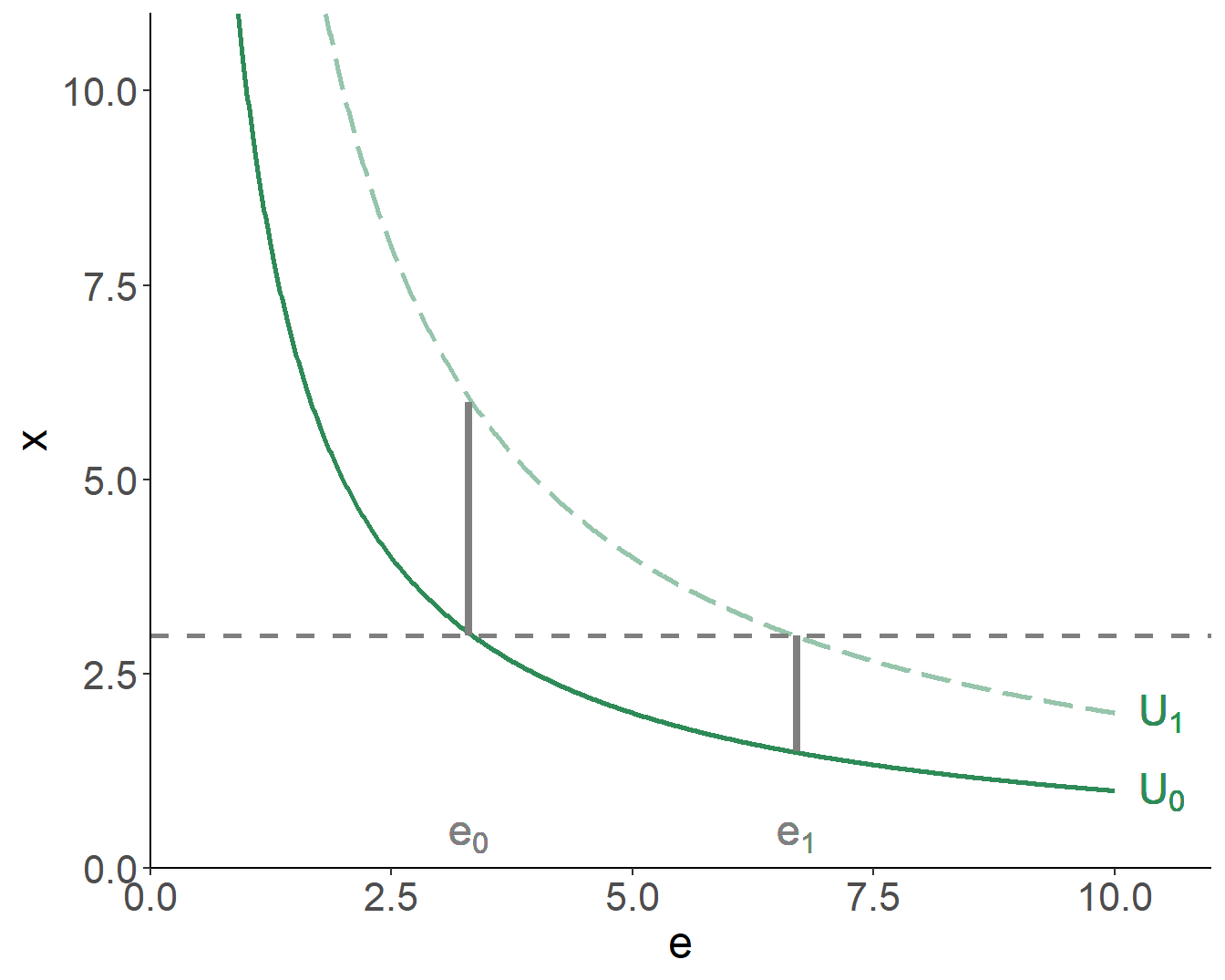
Figure 2.2: WTP vs WTA
As seen, WTA \(>\) WTP, which is the result of the indifference curves being convex to the origin, implying that as an individual decreases consumption of an environmental good, larger amounts of the market good are required to keep utility unchanged. This result is driven by the substantial change in the environmental good, otherwise—within a smaller region of the graph—indifference curves would be nearly linear, resulting in approximately equal WTP and WTA measures.
References
Adamowicz, Wiktor, Peter Boxall, Michael Williams, and Jordan Louviere. 1998. “Stated Preference Approaches for Measuring Passive Use Values: Choice Experiments and Contingent Valuation.” American Journal of Agricultural Economics 80 (1): 64–75.
Kolstad, Charles D. 2010. Environmental Economics. 2nd ed. Oxford University Press.